Probability Density Functions:
PDF File,View to Click Hear:

Probability Density Functions:
Probability density function:
From Wikipedia, the free encyclopedia
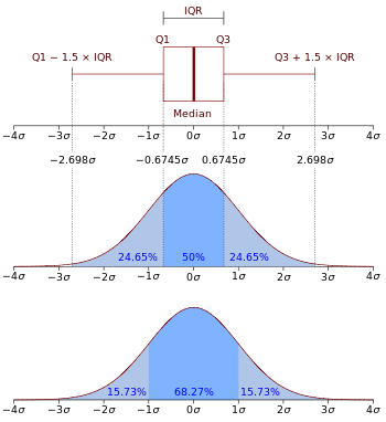
Boxplot and probability density function of a normal distributionN(0, σ2).
In probability theory, a probability density function (pdf), or density of a continuous random variable, is a function that describes the relative likelihood for this random variable to take on a given value. The probability for the random variable to fall within a particular region is given by the integral of this variable’s density over the region. The probability density function is nonnegative everywhere, and its integral over the entire space is equal to one.
The terms "probability distribution function"[1] and "probability function"[2] have also sometimes been used to denote the probability density function. However, this use is not standard among probabilists and statisticians. In other sources, "probability distribution function" may be used when the probability distribution is defined as a function over general sets of values, or it may refer to the cumulative distribution function, or it may be a probability mass function rather than the density. Further confusion of terminology exists because density function has also been used for what is here called the "probability mass function"
From Wikipedia, the free encyclopedia
Boxplot and probability density function of a normal distributionN(0, σ2).
In probability theory, a probability density function (pdf), or density of a continuous random variable, is a function that describes the relative likelihood for this random variable to take on a given value. The probability for the random variable to fall within a particular region is given by the integral of this variable’s density over the region. The probability density function is nonnegative everywhere, and its integral over the entire space is equal to one.
The terms "probability distribution function"[1] and "probability function"[2] have also sometimes been used to denote the probability density function. However, this use is not standard among probabilists and statisticians. In other sources, "probability distribution function" may be used when the probability distribution is defined as a function over general sets of values, or it may refer to the cumulative distribution function, or it may be a probability mass function rather than the density. Further confusion of terminology exists because density function has also been used for what is here called the "probability mass function"
Absolutely continuous univariate distributionsA probability density function is most commonly associated with absolutely continuous univariate distributions. A random variable X has density f, where f is a non-negative Lebesgue-integrablefunction, if:
Hence, if F is the cumulative distribution function of X, then:
and (if f is continuous at x)
Intuitively, one can think of f(x) dx as being the probability of X falling within the infinitesimal interval [x, x + dx].
Formal definition(This definition may be extended to any probability distribution using the measure-theoretic definition of probability.)
A random variable X with values in a measure space (usually Rn with the Borel sets as measurable subsets) has as probability distribution the measure X∗P on : the densityof X with respect to a reference measure μ on is the Radon–Nikodym derivative:
That is, f is any measurable function with the property that:
for any measurable set .
DiscussionIn the continuous univariate case above, the reference measure is the Lebesgue measure. The probability mass function of a discrete random variable is the density with respect to the counting measure over the sample space (usually the set of integers, or some subset thereof).
Note that it is not possible to define a density with reference to an arbitrary measure (i.e. one can't choose the counting measure as a reference for a continuous random variable). Furthermore, when it does exist, the density is almost everywhere unique.
Further detailsUnlike a probability, a probability density function can take on values greater than one; for example, the uniform distribution on the interval [0, ½] has probability density f(x) = 2 for 0 ≤ x ≤ ½ andf(x) = 0 elsewhere.
The standard normal distribution has probability density
If a random variable X is given and its distribution admits a probability density function f, then the expected value of X (if it exists) can be calculated as
Not every probability distribution has a density function: the distributions of discrete random variables do not; nor does the Cantor distribution, even though it has no discrete component, i.e., does not assign positive probability to any individual point.
A distribution has a density function if and only if its cumulative distribution function F(x) is absolutely continuous. In this case: F is almost everywhere differentiable, and its derivative can be used as probability density:
If a probability distribution admits a density, then the probability of every one-point set {a} is zero; the same holds for finite and countable sets.
Two probability densities f and g represent the same probability distribution precisely if they differ only on a set of Lebesgue measure zero.
In the field of statistical physics, a non-formal reformulation of the relation above between the derivative of the cumulative distribution function and the probability density function is generally used as the definition of the probability density function. This alternate definition is the following:
If dt is an infinitely small number, the probability that X is included within the interval (t, t + dt) is equal to f(t) dt, or:
Link between discrete and continuous distributionsIt is possible to represent certain discrete random variables as well as random variables involving both a continuous and a discrete part with a generalized probability density function, by using theDirac delta function. For example, let us consider a binary discrete random variable taking −1 or 1 for values, with probability ½ each.
The density of probability associated with this variable is:
More generally, if a discrete variable can take n different values among real numbers, then the associated probability density function is:
where x1, …, xn are the discrete values accessible to the variable and p1, …, pn are the probabilities associated with these values.
This substantially unifies the treatment of discrete and continuous probability distributions. For instance, the above expression allows for determining statistical characteristics of such a discrete variable (such as its mean, its variance and its kurtosis), starting from the formulas given for a continuous distribution of the probability.
Families of densitiesIt is common for probability density functions (and probability mass functions) to be parametrized, i.e. containing unspecified parameters. For example, the normal distribution is normally parametrized in terms of the mean and the variance, denoted by and respectively, giving the family of densities
It is important to keep in mind the difference between the domain of a family of densities and the parameters of the family. Different values of the parameters describe different distributions. A given set of parameters describes a single distribution, and the domain is the actual random variable that this distribution describes. From the perspective of a given distribution, the parameters are constants, and factors in a density function that contain only parameters, but not variables in the domain, are part of the normalization factor of a distribution and outside the kernel of the distribution. Since the parameters are constants, reparameterizing a family of densities in terms of different parameters means simply substituting the new parameters into the formula in the obvious way. Changing the domain of a probability density, however, is trickier and requires more work: see the section below on change of variables.
Densities associated with multiple variablesFor continuous random variables X1, …, Xn, it is also possible to define a probability density function associated to the set as a whole, often called joint probability density function. This density function is defined as a function of the n variables, such that, for any domain D in the n-dimensional space of the values of the variables X1, …, Xn, the probability that a realisation of the set variables falls inside the domain D is
If F(x1, …, xn) = Pr(X1 ≤ x1, …, Xn ≤ xn) is the cumulative distribution function of the vector (X1, …, Xn), then the joint probability density function can be computed as a partial derivative
Marginal densitiesFor i=1, 2, …,n, let fXi(xi) be the probability density function associated with variable Xi alone. This is called the “marginal” density function, and can be deduced from the probability density associated with the random variables X1, …, Xn by integrating on all values of the n − 1 other variables:
IndependenceContinuous random variables X1, …, Xn admitting a joint density are all independent from each other if and only if
CorollaryIf the joint probability density function of a vector of n random variables can be factored into a product of n functions of one variable
(where each fi is not necessarily a density) then the n variables in the set are all independent from each other, and the marginal probability density function of each of them is given by
ExampleThis elementary example illustrates the above definition of multidimensional probability density functions in the simple case of a function of a set of two variables. Let us call a 2-dimensional random vector of coordinates (X, Y): the probability to obtain in the quarter plane of positive x and y is
Dependent variables and change of variablesIf the probability density function of a random variable X is given as fX(x), it is possible (but often not necessary; see below) to calculate the probability density function of some variable Y = g(X). This is also called a “change of variable” and is in practice used to generate a random variable of arbitrary shape fg(X) = fY using a known (for instance uniform) random number generator.
If the function g is monotonic, then the resulting density function is
Here g−1 denotes the inverse function.
This follows from the fact that the probability contained in a differential area must be invariant under change of variables. That is,
or
For functions which are not monotonic the probability density function for y is
where n(y) is the number of solutions in x for the equation g(x) = y, and g−1k(y) are these solutions.
It is tempting to think that in order to find the expected value E(g(X)) one must first find the probability density fg(X) of the new random variable Y = g(X). However, rather than computing
one may find instead
The values of the two integrals are the same in all cases in which both X and g(X) actually have probability density functions. It is not necessary that g be a one-to-one function. In some cases the latter integral is computed much more easily than the former.
Multiple variablesThe above formulas can be generalized to variables (which we will again call y) depending on more than one other variable. f(x1, …, xn) shall denote the probability density function of the variables that y depends on, and the dependence shall be y = g(x1, …, xn). Then, the resulting density function is
where the integral is over the entire (n-1)-dimensional solution of the subscripted equation and the symbolic dV must be replaced by a parametrization of this solution for a particular calculation; the variables x1, …, xn are then of course functions of this parametrization.
This derives from the following, perhaps more intuitive representation: Suppose x is an n-dimensional random variable with joint density f. If y = H(x), where H is a bijective, differentiable function, then y has density g:
with the differential regarded as the Jacobian of the inverse of H, evaluated at y.
Using the delta-function (and assuming independence) the same result is formulated as follows.
If the probability density function of independent random variables Xi, i = 1, 2, …n are given as fXi(xi), it is possible to calculate the probability density function of some variableY = G(X1, X2, …Xn). The following formula establishes a connection between the probability density function of Y denoted by fY(y) and fXi(xi) using the Dirac delta function:
Sums of independent random variablesSee also: Convolution and List of convolutions of probability distributions
The probability density function of the sum of two independent random variables U and V, each of which has a probability density function, is the convolution of their separate density functions:
It is possible to generalize the previous relation to a sum of N independent random variables, with densities U1, …, UN:
This can be derived from a two-way change of variables involving Y=U+V and Z=V, similarly to the example below for the quotient of independent random variables.
Products and quotients of independent random variablesSee also: Product distribution and Ratio distribution
Given two independent random variables U and V, each of which has a probability density function, the density of the product Y=UV and quotient Y=U/V can be computed by a change of variables.
[edit]Example: Quotient distributionTo compute the quotient Y=U/V of two independent random variables U and V, define the following transformation:
Then, the joint density p(Y,Z) can be computed by a change of variables from U,V to Y,Z, and Y can be derived by marginalizing out Z from the joint density.
The inverse transformation is
The Jacobian matrix of this transformation is
Thus:
And the distribution of Y can be computed by marginalizing out Z:
Note that this method crucially requires that the transformation from U,V to Y,Z be bijective. The above transformation meets this because Z can be mapped directly back to V, and for a given Vthe quotient U/V is monotonic. This is similarly the case for the sum U+V, difference U-V and product UV.
Exactly the same method can be used to compute the distribution of other functions of multiple independent random variables.
[edit]Example: Quotient of two standard normalsGiven two standard normal variables U and V, the quotient can be computed as follows. First, the variables have the following density functions:
We transform as described above:
This leads to:
This is a standard Cauchy distribution.
See also
^ Taken the references from Wikipedia 08 Sep,2012
^ Taken the references from Youtub.com , 2012
Hence, if F is the cumulative distribution function of X, then:
and (if f is continuous at x)
Intuitively, one can think of f(x) dx as being the probability of X falling within the infinitesimal interval [x, x + dx].
Formal definition(This definition may be extended to any probability distribution using the measure-theoretic definition of probability.)
A random variable X with values in a measure space (usually Rn with the Borel sets as measurable subsets) has as probability distribution the measure X∗P on : the densityof X with respect to a reference measure μ on is the Radon–Nikodym derivative:
That is, f is any measurable function with the property that:
for any measurable set .
DiscussionIn the continuous univariate case above, the reference measure is the Lebesgue measure. The probability mass function of a discrete random variable is the density with respect to the counting measure over the sample space (usually the set of integers, or some subset thereof).
Note that it is not possible to define a density with reference to an arbitrary measure (i.e. one can't choose the counting measure as a reference for a continuous random variable). Furthermore, when it does exist, the density is almost everywhere unique.
Further detailsUnlike a probability, a probability density function can take on values greater than one; for example, the uniform distribution on the interval [0, ½] has probability density f(x) = 2 for 0 ≤ x ≤ ½ andf(x) = 0 elsewhere.
The standard normal distribution has probability density
If a random variable X is given and its distribution admits a probability density function f, then the expected value of X (if it exists) can be calculated as
Not every probability distribution has a density function: the distributions of discrete random variables do not; nor does the Cantor distribution, even though it has no discrete component, i.e., does not assign positive probability to any individual point.
A distribution has a density function if and only if its cumulative distribution function F(x) is absolutely continuous. In this case: F is almost everywhere differentiable, and its derivative can be used as probability density:
If a probability distribution admits a density, then the probability of every one-point set {a} is zero; the same holds for finite and countable sets.
Two probability densities f and g represent the same probability distribution precisely if they differ only on a set of Lebesgue measure zero.
In the field of statistical physics, a non-formal reformulation of the relation above between the derivative of the cumulative distribution function and the probability density function is generally used as the definition of the probability density function. This alternate definition is the following:
If dt is an infinitely small number, the probability that X is included within the interval (t, t + dt) is equal to f(t) dt, or:
Link between discrete and continuous distributionsIt is possible to represent certain discrete random variables as well as random variables involving both a continuous and a discrete part with a generalized probability density function, by using theDirac delta function. For example, let us consider a binary discrete random variable taking −1 or 1 for values, with probability ½ each.
The density of probability associated with this variable is:
More generally, if a discrete variable can take n different values among real numbers, then the associated probability density function is:
where x1, …, xn are the discrete values accessible to the variable and p1, …, pn are the probabilities associated with these values.
This substantially unifies the treatment of discrete and continuous probability distributions. For instance, the above expression allows for determining statistical characteristics of such a discrete variable (such as its mean, its variance and its kurtosis), starting from the formulas given for a continuous distribution of the probability.
Families of densitiesIt is common for probability density functions (and probability mass functions) to be parametrized, i.e. containing unspecified parameters. For example, the normal distribution is normally parametrized in terms of the mean and the variance, denoted by and respectively, giving the family of densities
It is important to keep in mind the difference between the domain of a family of densities and the parameters of the family. Different values of the parameters describe different distributions. A given set of parameters describes a single distribution, and the domain is the actual random variable that this distribution describes. From the perspective of a given distribution, the parameters are constants, and factors in a density function that contain only parameters, but not variables in the domain, are part of the normalization factor of a distribution and outside the kernel of the distribution. Since the parameters are constants, reparameterizing a family of densities in terms of different parameters means simply substituting the new parameters into the formula in the obvious way. Changing the domain of a probability density, however, is trickier and requires more work: see the section below on change of variables.
Densities associated with multiple variablesFor continuous random variables X1, …, Xn, it is also possible to define a probability density function associated to the set as a whole, often called joint probability density function. This density function is defined as a function of the n variables, such that, for any domain D in the n-dimensional space of the values of the variables X1, …, Xn, the probability that a realisation of the set variables falls inside the domain D is
If F(x1, …, xn) = Pr(X1 ≤ x1, …, Xn ≤ xn) is the cumulative distribution function of the vector (X1, …, Xn), then the joint probability density function can be computed as a partial derivative
Marginal densitiesFor i=1, 2, …,n, let fXi(xi) be the probability density function associated with variable Xi alone. This is called the “marginal” density function, and can be deduced from the probability density associated with the random variables X1, …, Xn by integrating on all values of the n − 1 other variables:
IndependenceContinuous random variables X1, …, Xn admitting a joint density are all independent from each other if and only if
CorollaryIf the joint probability density function of a vector of n random variables can be factored into a product of n functions of one variable
(where each fi is not necessarily a density) then the n variables in the set are all independent from each other, and the marginal probability density function of each of them is given by
ExampleThis elementary example illustrates the above definition of multidimensional probability density functions in the simple case of a function of a set of two variables. Let us call a 2-dimensional random vector of coordinates (X, Y): the probability to obtain in the quarter plane of positive x and y is
Dependent variables and change of variablesIf the probability density function of a random variable X is given as fX(x), it is possible (but often not necessary; see below) to calculate the probability density function of some variable Y = g(X). This is also called a “change of variable” and is in practice used to generate a random variable of arbitrary shape fg(X) = fY using a known (for instance uniform) random number generator.
If the function g is monotonic, then the resulting density function is
Here g−1 denotes the inverse function.
This follows from the fact that the probability contained in a differential area must be invariant under change of variables. That is,
or
For functions which are not monotonic the probability density function for y is
where n(y) is the number of solutions in x for the equation g(x) = y, and g−1k(y) are these solutions.
It is tempting to think that in order to find the expected value E(g(X)) one must first find the probability density fg(X) of the new random variable Y = g(X). However, rather than computing
one may find instead
The values of the two integrals are the same in all cases in which both X and g(X) actually have probability density functions. It is not necessary that g be a one-to-one function. In some cases the latter integral is computed much more easily than the former.
Multiple variablesThe above formulas can be generalized to variables (which we will again call y) depending on more than one other variable. f(x1, …, xn) shall denote the probability density function of the variables that y depends on, and the dependence shall be y = g(x1, …, xn). Then, the resulting density function is
where the integral is over the entire (n-1)-dimensional solution of the subscripted equation and the symbolic dV must be replaced by a parametrization of this solution for a particular calculation; the variables x1, …, xn are then of course functions of this parametrization.
This derives from the following, perhaps more intuitive representation: Suppose x is an n-dimensional random variable with joint density f. If y = H(x), where H is a bijective, differentiable function, then y has density g:
with the differential regarded as the Jacobian of the inverse of H, evaluated at y.
Using the delta-function (and assuming independence) the same result is formulated as follows.
If the probability density function of independent random variables Xi, i = 1, 2, …n are given as fXi(xi), it is possible to calculate the probability density function of some variableY = G(X1, X2, …Xn). The following formula establishes a connection between the probability density function of Y denoted by fY(y) and fXi(xi) using the Dirac delta function:
Sums of independent random variablesSee also: Convolution and List of convolutions of probability distributions
The probability density function of the sum of two independent random variables U and V, each of which has a probability density function, is the convolution of their separate density functions:
It is possible to generalize the previous relation to a sum of N independent random variables, with densities U1, …, UN:
This can be derived from a two-way change of variables involving Y=U+V and Z=V, similarly to the example below for the quotient of independent random variables.
Products and quotients of independent random variablesSee also: Product distribution and Ratio distribution
Given two independent random variables U and V, each of which has a probability density function, the density of the product Y=UV and quotient Y=U/V can be computed by a change of variables.
[edit]Example: Quotient distributionTo compute the quotient Y=U/V of two independent random variables U and V, define the following transformation:
Then, the joint density p(Y,Z) can be computed by a change of variables from U,V to Y,Z, and Y can be derived by marginalizing out Z from the joint density.
The inverse transformation is
The Jacobian matrix of this transformation is
Thus:
And the distribution of Y can be computed by marginalizing out Z:
Note that this method crucially requires that the transformation from U,V to Y,Z be bijective. The above transformation meets this because Z can be mapped directly back to V, and for a given Vthe quotient U/V is monotonic. This is similarly the case for the sum U+V, difference U-V and product UV.
Exactly the same method can be used to compute the distribution of other functions of multiple independent random variables.
[edit]Example: Quotient of two standard normalsGiven two standard normal variables U and V, the quotient can be computed as follows. First, the variables have the following density functions:
We transform as described above:
This leads to:
This is a standard Cauchy distribution.
See also
- Probability mass function
- Likelihood function
- Density estimation
- Secondary measure
- List of probability distributions
^ Taken the references from Wikipedia 08 Sep,2012
^ Taken the references from Youtub.com , 2012
